Create a new model

First go to the menu STATISTICAL METHODS and select the option Nowcasting. Select the type of nowcasting model desired. For example, “dynamic factor models”.

Here we show how to specify a model, in a few simple steps:

1. Upload the data and drag and drop it to the model

As suggested earlier, the data can be uploaded from various sources. Select the sheets that contains your data and copy each series or the whole sheet into the model space (use the drag and drop command).

Your newly created nowcasting model has two factors by default. Below, we describe the options to link the data to those two underlying factors. We also describe how to change the number of factors and other options.

2. Model specification details

The so-called state-space representation of the factor model is written as follows:

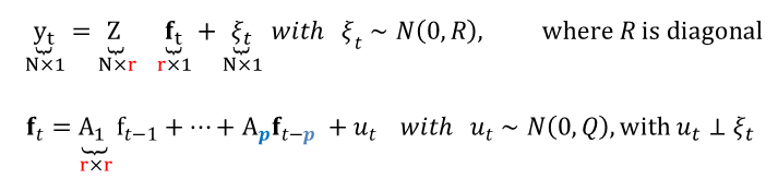
where the measurement equation links the N observables to the r underlying factors. Those factors, as shown in the second equation, follow a VAR of order p (transition equation). This representation is valid in the case of missing observations or when monthly and quarterly variables are combined. In the latter case, it is simply assumed that the quarterly values are observed every three months.

2.1. Define the measurement equation

In this example we have variables observed at the monthly and quarterly frequencies. There is the option to transform the series in multiple ways, including first differences or seasonal adjustment. The likelihood of the model which is will be important for the estimation, will be given by the transformed data. However, the forecasts will be calculated for the raw data.

The link between the transformed time series and the factors can be very sophisticated. Three options are possible for the moment:

• Variables expressed in terms of monthly growth rates can be linked to a factor representing the underlying monthly growth rate of the economy if “M” is selected

  

• Monthly or quarterly variables that are correlated with the the underlying quarterly growth rate of the economy can be linked to a weighted average of the factors representing the underlying monthly growth rate of the economy. Such a weighted average is meant to approximate quarterly growth rates, and it is implemented by selecting “Q” (see econometric model):

  

• Variables representing yearly growth rates are linked to a moving average of the factors that represent the underlying monthly growth rate of the economy_. Such a weighted average is meant to approximate the growth rate of a year, and it is implemented by selecting “Y” (see econometric model):

  

• The variables can also be linked to the cumulative sum of the last 12 monthly factors. If the model is designed in such a way that the monthly factors represent monthly growth rates, the resulting cumulative sum boils down to the year-on-year growth rate. Thus, variables expressed in terms of year-on-year growth rates or surveys that are correlated with the year-on-year growth rates of the reference series should be linked to the factors using this link (see econometric model):

  

• Variables representing expected changes over a forecast horizon (see econometric model)

  

• Variables represening forecasts for a precise horizon (see econometric model)

  

The factor loading structure can incorporate zero restrictions. Users should simply select which factors load on which variables. The following example helps to define a measurement equation for a very simple model for nowcasting German GDP:

2.2. Define the transition equation

The so-called transition equation is a representation of the r underlying factors in terms of a vector autoregressive model of order p. Both parameters can be determined by clicking on the tools option of Model tab.

The first unobserved factors in the sample is assumed either to be equal to zero or be consistent with a normal distribution with mean zero and a variance consistent with the unconditional variance of the VAR.

2.3. Save your workspace and model specifications

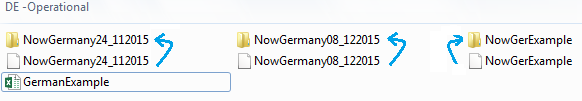
• The workspace can be saved by clicking on the FILE menu and selecting “save as”. Let’s first save the workspace with the name “NowGermany_24_11_2015”, in reference to today’s date.

• The name of our new model residing in our workspace (“Dfm1”, by default) can be easily changed by applying the right click command. Select “Rename”. Call it “Model r=2, p=3”, in reference to the fact that the correlation among all variables is exclusively due to r=2 factors, which follow a VAR(p) of order p=3.

3. Clone the previous model and improve it

As shown in the video, one may want to build a new model with identical properties as the previous one, but with one extra factor that loads on a variable that could be important for the German business cycle (this hypothesis can be tested). Go to the workspace window and right click on the model you want to modify. Select “Clone”.

You can see that a new model will be added to the list of models that already exist inside your workspace. Proceed as before (right click) with this new model, and select the option “Rename”. Call it “Model r=3, p=3”, in reference to the fact that it has now three factors following a VAR(3).

4. Where is all that information stored ?

An XML file with name “NowGermany_24_11_2015” is created. Such a file can be opened with JDemetra+. The file will access a folder with the same name that contain the two models we have specified, including the data.