Reading news
Here we show how to interpret revisions in the forecasts in terms of surprises in new data releases. The illustrations of this page have been constructed using with the model developed by Basselier, De-Antonio-Liedo and Langenus (2016). Download the paper for an explanation of the methodology and the relevant references.
The concept
This figure represents in a simplified manner two consecutive information sets and the weights associated to the news. Note that the weight’s subindex corresponds to each one of the pieces of news, while the upper index h refers to the target variable, which is next quarter’s GDP growth. In practice, the updated information set may contain not only additional data points but also revisions for past values.
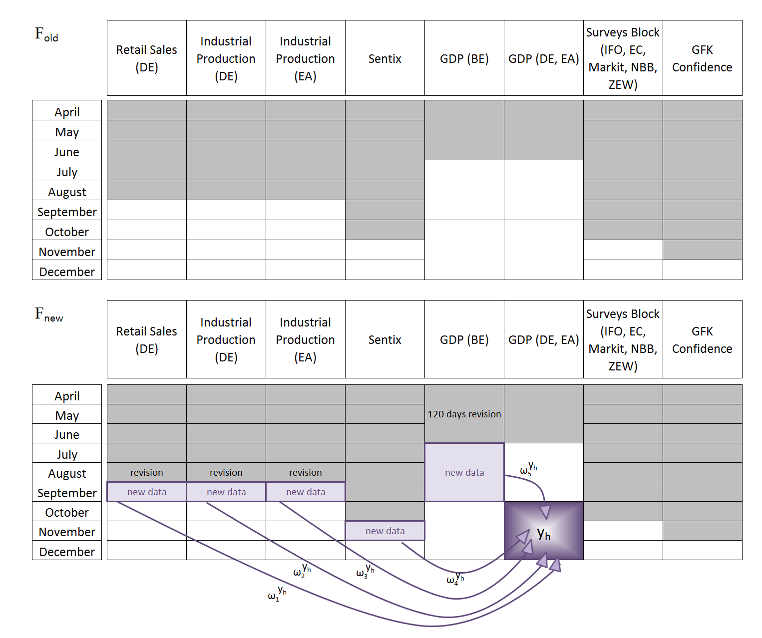
All those new data releases (and data revisions) are converted into news by the model and those news, which is the difference between the released value and the one expected by the model, will determine the extent to which the forecasts are revised. In this figure, we represent the mapping from this news onto the forecast for GDP.
Each piece of news contriutes to the forecasting updates via the weight, which is specific to the variable we want to forecast and the time horizon, as shown in the
diagram. The same formulation applies for updating any other variable and foreasting horizon,
but we need to use a slightly more precise notation:
where the subindex \(k\) refers in general to a particular element of the vector of observations and \(t+h\) refers to time dimension. Thus, the weights that play a role at updating \(y_{k,t+h}\) will also be indexed by \(k\) and \(t+h\). The third subindex \(j\) associated to the weights refers to the news. The different news components are indexed by \(j=1,\ldots, J\) independently on the variable \(i_{j}\) and time horizon \(t_{j}\) to which they refer.
The weights are given by the Kalman gain
Let’s include all news in one vector: \(\begin{equation} \left\{\mathcal{F}^{refreshed} - \mathcal{F}^{old} \right\}\equiv \mathcal{I} = \left[ \begin{array}{c} y_{(i,t)_{1}} - E[y_{(i,t)_{1}}|\mathcal{F}^{old}] \\ \vdots \\ y_{(i,t)_{J}} - E[y_{(i,t)_{J}}|\mathcal{F}^{old}] \end{array} \right] \end{equation}\)
The weights associated to each piece of news are calculated as follows:
\[\begin{equation} \left[ w^{k,h}_{1} \ldots w^{k,h}_{J}\right] = E[y_{k,t+h}\mathcal{I}^{'}]E[\mathcal{I}\mathcal{I}^{'}]^{-1} \end{equation}\]In order to calculate the weights, we use the Kalman smoother for the determination of the precision matrices, which are an essential part of the formula:
- The covariance between the target variable and the news vector has the following form:
- The covariance of the news vector can be written as follows:
As shown in the examples, the graphical interface proposed allows users to understand how the forecasting revisions can be decomposed in terms of the news components for the various indicators. The news with the largest impact will be quickly identified in a barchart.
Steps: Archive, Refresh and Update forecasts
Open the workspace that contains your model and double click on it. Only one model can be activated at a time and its name will appear in the menu bar next to “statistical models”. By clicking on its name, you will have the following options:
RefreshArchiveRemove last archiveUnlock
Here, we assume that we are happy with the model and we want to start using it. Before finishing the analysis and exiting the program, click on Archive and, very important, save the workspace. The Archive action, which freezes the model and the data, needs to be saved so that it can be accessed next time you want the model to update the forecasts on the basis of new data. In our examples, the model was archived at the end of November of 2016.
One month later, at the end of December of 2016, our dataset is updated. In order to make the model read that new data and update the forecasts, we simply have to click on the Refresh option.
Once this is done, we can go to the tab NEWS and click on Weights to visualize the updated forecast together with the previous one. The weight of each piece of news at updating the forecast for each period, which was represented in the equation above, is displayed in the form of a table. It is wise to save the updated workspace under a name that contains the date, e.g. Model_25November2015. If you do this every two weeks, you will accumulate many different workshops that you can use to keep track of your history of updates.
Also within the tab NEWS, you can click on Impacts to see how the forecasting revision, i.e. the new forecast minus the previous one, is decomposed in terms of the news. Thus, the table contains the impacts, which are given by the weights of the news times their size. Below, you will find two examples where we analyse the contribution of the different news at forecasting for both German GDP and the euro area aggregate.