Maximum-likelihood estimation of a mixed-frequency dynamic factor model with missing observations

1. Options

The estimation options are illustrated here using the following workspace (example based on Banbura and Modugno, 2014)

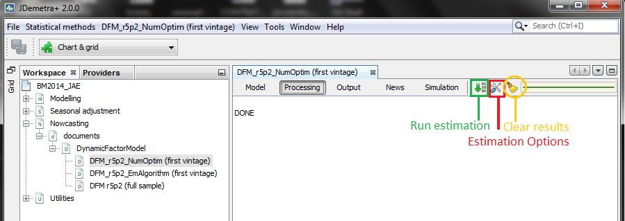
By clicking on the tools option of PROCESSING tab, you can combine select the options to estimate the parameters. Once selected, you can click on the estimation icon to proceed with the estimation. The estimation results can be deleted by clicking on the clear icon . This action ensures that previous results, including the sample means, are completely erased and are not used in the estimation as starting values.

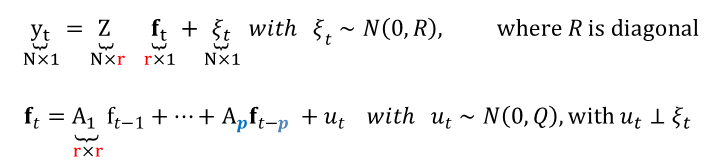
Numerical optimization and the EM algorithm play the most important role, and they can be combined. Let’s look at two different ways to estimate the large dynamic factor model for the euro area described before, which has N=101 variables, r=5 factors and two p=2 lags:

Numerical Optimization

• STEP 1 : Principal components (PC) to extract the factors and run OLS regressions to get Z, R,A, and Q
• STEP 2 :Use PC as starting value of a numerical optimization procedure (Levenberg-Marquardt) for the pseudo-likelihood (p=1). Not necessary to iterate until convergence: in this exaple, 15 iterations.
• STEP 3 : Use the estimator obtained in the previous step as a starting value of the numerical optimization procedure for the true likelihood (p=2 in this example). The algorithm stops when the percentage likelihood does not increase by more than 1.0E-9. This value can be changed.
  

Expectations-Maximization algorithm

• STEP 1 : Principal components (PC) to extract the factors and run OLS regressions to get Z, R,A, and Q
• STEP 2 :Use PC as an initial condition for the EM algorithm and run it until the percentage likelihood does not increase by more than 1.0E-9. This algorithm, considers the analytical form of the first order conditions of the (expected) likelihood maximization problem, may converge very slowly when it is exploring the neighbourhood of the maximum likelihood solution.
• STEP 3 : This final step may help to converge faster, but the results may be driven by the outcome of the previous EM step. We use the estimator obtained in STEP 2 as a starting value of the optimization procedure for the likelihood. Here, simplified model iterations is set to zero so that the likelihood continues improving until convergence.

Some tips

• Estimation by blocks: The model parameters are divided in two blocks: {Z,R} and {A1,…,Ap,Q}. While the EM algorithm requires one iteration per block, the numerical optimization allows us to set the number of iterations desired per block, which is equal to 5 in this example.

• Mixed estimation: The mixed estimation option alternates between the iterations for the VAR block: {A1,…,Ap,Q} alone and simultaneous iterations for the two blocks.

• Principal components. Both estimation options described here start with parameter values obtained with principal components.

• Use EM before Numerical Using the EM results as starting values for numerical optimization, as illustrated here, is standard practice, but not the other way round. A final run of the EM algorithm is also possible, but useless in practice.

• No rules of thumb. For very large models, it may be useful to use the EM algorithm before the numerical optimization procedure. However, for the relatively large model used here (101 variables available until 1999, r=5 and p=2), the numerical optimization strategy has proved to be more efficient, although this difference disappears when the Great Recession is included in the estimation.

• Running the model without re-estimating the parameters. When all the options inside tools are checked out, the model parameters are not re-estimated by clicking on the estimation icon . This only triggers the Kalman filter and smoother to update the factors without any modification in the model parameters. The estimation options become unchecked by default when you refresh your data. To put it simply, consider the factors as a weighted average of the data. When new data arrives, the factors can be recalculated using the same weights. This leads to new forecasts, even if the model parameters have not been re-estimated.

2. Example

The following video shows how to proceed with the estimation of a large dynamic factor model with r=7 factors and p=3 lags accounting for the dynamics of N=101 indicators. This model has a relatively large number of parameters that have to be estimated. Also, the size of the state equation is very large (7x3x5=105 )because quarterly variables in the measurement equation load on a weighted average of the last five factors.

The information displayed shows a continuous increase in the likelihood, with large improvements during the numerical optimization process, particularly at the first step of each block of five iterations.

Estimation speed depends on the size of the model. Models with one or two factors will be estimated in less than five seconds, also when the number of variables is large. However, the estimation of models like the one used in this example may take about 30 minutes to converge.