Trading days
Definition of trading days effects
We consider in this document the regression variables that can be defined in JD+ to model trading days effects. We call them hereafter “trading days variables (TD)”.
A natural way for modelling trading days effects consists in distributing the days of each period in different groups. The regression variable corresponding to a type of day (a group) is simply defined by the number of days it contains for each period. Usual classifications are:
- Trading days (7 groups): each day of the week defines a group (Mondays…Sundays)
- Working days (2 groups): week days and weekends
But we could also consider:
- 3 groups: week days (Mondays->Fridays), Saturdays, Sundays; that solution will be called TD3 hereafter …
The definition of a group could involve partial days. For instance, we could consider that one half of Saturdays belong to week days and the second half to weekends
Specific holidays are often handled as Sundays: they go to the group that contains the Sundays (or more generally to the group corresponding to “non-working days”), but they also could be considered separately: for instance 8 groups: trading days (outside specific holidays) + specific holidays.
Example:
Week days + Saturdays + Sundays
| Total | Week days | Saturdays | Sundays | |
|---|---|---|---|---|
| Jan-2017 | 31 | 22 | 4 | 5 |
| Feb-2017 | 28 | 20 | 4 | 4 |
| Mar-2017 | 31 | 23 | 4 | 4 |
| Apr-2017 | 30 | 20 | 5 | 5 |
| May-2017 | 31 | 23 | 4 | 4 |
| Jun-2017 | 30 | 22 | 4 | 4 |
| Jul-2017 | 31 | 21 | 5 | 5 |
| Aug-2017 | 31 | 23 | 4 | 4 |
| Sep-2017 | 30 | 21 | 5 | 4 |
Mean and seasonal effects of TD
The definition proposed above will lead to regression variables that have a mean effect and a seasonal effect. In the usual decomposition of a series, the mean effect (independent of the period) should be allocated to the trend-cycle component and the fixed seasonal effect (dependent of the period, 0 on average) should be affected to the corresponding component. So, the actual trading days effect should only contain effects that don’t belong to the other components. Such a choice is just a sensible convention. By mean effect and seasonal effect, we consider in JDemetra+ long term theoretical effects and not effects computed on the time span of the considered series (which should be continuously revised). To correct the variables for their long term mean and seasonal effects, we just have to remove the long term means of each period. We apply below those corrections for the week days of TD3 (or TD2). If we consider the variable “week days” in TD3 (or TD2), we have:
| Period (p) | Average number of week days | Average number of Saturdays/Sundays |
|---|---|---|
| Jan | 31*5/7=22.1429 | 31/7=4.4286 |
| Feb | 28.25*5/7=20.1786 | 28.25/7=4.0357 |
| Mar | 31*5/7=22.1429 | 31/7=4.4286 |
| Apr | 30*5/7=21.4286 | 30/7=4.2857 |
| May | 31*5/7=22.1429 | 31/7=4.4286 |
| Jun | 30*5/7=21.4286 | 30/7=4.2857 |
| Jul | 31*5/7=22.1429 | 31/7=4.4286 |
| Aug | 31*5/7=22.1429 | 31/7=4.4286 |
| Sep | 30*5/7=21.4286 | 30/7=4.2857 |
For a given time span, the actual “trading days effects” is then easily derived.
| Time period (t) | # Week days | TD effect of week days | # Sundays | TD effect of Sundays |
|---|---|---|---|---|
| Jan-2017 | 22 | -0.1429 | 5 | 0.5714 |
| Feb-2017 | 20 | -0.1786 | 4 | -0.0357 |
| Mar-2017 | 23 | 0.8571 | 4 | -0.4286 |
| Apr-2017 | 20 | -1.4286 | 5 | 0.7143 |
| May-2017 | 23 | 0.8571 | 4 | -0.4286 |
| Jun-2017 | 22 | 0.5714 | 4 | -0.2857 |
| Jul-2017 | 21 | -1.1429 | 5 | 0.5714 |
| Aug-2017 | 23 | 0.8571 | 4 | -0.4286 |
| Sep-2017 | 21 | -0.4286 | 4 | -0.2857 |
Contrasts
The standard way to deal with trading days effects is based on contrasts. This is also the case in JD+. Contrasts are defined as the (weighted) differences between the number of days in the groups of trading days and a “reference” group, which is by convention the “non-working” days (Sundays, week-ends…). For instance:
- TD7: #Mondays - #Sundays, …, #Saturdays - #Sundays.
- TD3: #Week days – 5 * #Sundays, #Saturdays - #Sundays
- TD2: #Week days – 5/2 * (#Saturdays + #Sundays)
In the standard case, the weights of the contrasts, based on the number of days in each group, eliminate the mean and seasonal effects. However, this is no longer the case when we consider specific holidays.
The use of contrasts in regression models leads to several drawbacks.
For instance, in the case of TD7, we have:
\[c_1 \left( \# Mon - \# Sun \right) + \cdots c_6 \left( \# Sat - \# Sun \right)\] \[= c_1 \# Mon + \cdots + c_6 \# Sat - \left( c_1 + \cdots + c_6 \right) \# Sun\]So, the coefficient related to the Sundays is the opposite of the sum of the other coefficients, so that the sum of all coefficients is 0.
Handling of specific holidays
We consider in JD+ the following type of holidays:
- Fixed day, corresponding to a fixed date in the year (for instance July, 21 for Belgium, New Year, Christmas).
- Easter related days, corresponding to days that are defined in relation to Easter (Easter +- n days; example: Ascension…)
- Fixed week days, corresponding to a fixed day in a given week of a given month (Labour Day…)
From a conceptual point of view, specific holidays are handled exactly the same way as the other days. We just have to decide in which group they are put. Usually - and it is the convention used in JD+, they are handled has Sundays. Of course, except if the holiday falls on a Sunday, we have to correct both the group that should have contained the holiday and the group that contains the Sundays.
The trickiest aspect of specific holidays is the way they impact on the mean and the seasonal effects of TDs. We consider below the seasonal corrections that should be applied on the Mondays…Sundays following the kind of holidays.
The corrections are applied to the period(s) that can contain the holiday.
Fixed day
The probability that the holiday falls on a Sunday is 1/7 (and the same for the other days). The probability to have 1 Sunday more is 6/7. The effect on the means for the period that contains the date is (the correction on the calendar effect has the opposite sign):
| Sundays | Other days | Contrasts |
| +6/7 | -1/7 | -1 |
We show below the impact of such day – 21 July, national holiday of Belgium – on TD7 (contrasts) 21 July falls on a Friday in 2017 and on a Sunday in 2019.
| Monday | Tuesday | Wednesday | Thursday | Friday | Saturday | |
|---|---|---|---|---|---|---|
| July 2017 | ||||||
| Default TD | 0 | -1 | -1 | -1 | -1 | 0 |
| Belgium calendar (not corrected) | -1 | -2 | -2 | -2 | -3 | -1 |
| Long term correction | +1 | +1 | +1 | +1 | +1 | +1 |
| Belgium calendar | 0 | -1 | -1 | -1 | -2 | 0 |
| July 2019 | ||||||
| Default TD | +1 | +1 | +1 | 0 | 0 | 0 |
| Belgium calendar (not corrected) | +1 | +1 | +1 | 0 | 0 | 0 |
| Long term correction | +1 | +1 | +1 | +1 | +1 | +1 |
| Belgium calendar | +2 | +2 | +2 | +1 | +1 | +1 |
Easter related days
Easter related days always fall the same week day (X). However, they can fall during different periods (months or quarters). Suppose that, taking into account the distribution of the dates for Easter, the probability that the holiday falls during the period m (m+1) is p (1-p). Then, the effects on the seasonal means are:
| Period | Sundays | Days X | Others days | Contrast X | Other contrasts |
|---|---|---|---|---|---|
| m | +p | -p | 0 | -2*p | -p |
| m+1 | +(1-p) | -(1-p) | 0 | -2*(1-p) | -(1-p) |
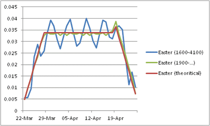
The distribution of the dates for Easter might be approximated in different ways.
A first solution consists in using some well-known algorithms for computing Easter on a very long period. JDemetra+ provides the Meeus/Jones/Butcher’s and the Ron Mallen’s algorithms (they are identical till 4100).
Another approach consists in deriving a raw theoretical distribution based on the definition of Easter. It is the solution used for Easter related days. It is shortly explained below.
“Easter is the first Sunday after the full moon (the Paschal Full Moon) following the northern hemisphere’s vernal equinox. Ecclesiastically, the equinox is reckoned to be on 21 March (even though the equinox occurs, astronomically speaking, on 20 March in most years), and the “Full Moon” is not necessarily the astronomically correct date. Easter is delayed by 1 week if the full moon is on Sunday. The date of Easter therefore varies between 22 March and 25 April” (Wikipedia). Taking into account that an average lunar month is 29.53059 days, we can derive raw formulae for the approximated distribution of Easter (they don’t take into account the actual ecclesiastical moon calendar).
| date | probability |
|---|---|
| 22/3 | 1/7 * 1/29.53059 |
| 23/3 | 1/7 * 2/29.53059 |
| 24/3 | 1/7 * 3/29.53059 |
| 25/3 | 1/7 * 4/29.53059 |
| 26/3 | 1/7 * 5/29.53059 |
| 27/3 | 1/7 * 6/29.53059 |
| 28/3 | 1/29.53059 |
| 29/3 | 1/29.53059 |
| … | … |
| 8/4 | 1/29.53059 |
| 19/4 | 1/7 * (6 + 1.53059)/29.53059 |
| 20/4 | 1/7 * (5 + 1.53059)/29.53059 |
| 21/4 | 1/7 * (4 + 1.53059)/29.53059 |
| 22/4 | 1/7 * (3 + 1.53059)/29.53059 |
| 23/4 | 1/7 * (2 + 1.53059)/29.53059 |
| 24/4 | 1/7 * (1 + 1.53059)/29.53059 |
| 25/4 | 1/7 * 1.53059/29.53059 |
For example,
- The probability that Easter falls on 25/3 is computed as follows:
- Probability that 25/3 is a Sunday: 1/7
- Probability that the full moon is on 21/3… 24/3 is 5/29.53059
- The probability that Easter falls on 23/4 is computed as follows:
- Probability that 23/4 is a Sunday: 1/7
- Probability that the full moon is on 16/4, 17/4: 2/29.53059
- Probability that the full moon is on 18/4 1.53059/29.53059
The different solutions are presented below.
Fixed week days
Fixed week days always fall the same week day (X) and the same period. Their effect on the seasonal means is:
| Sundays | Days X | Others days |
|---|---|---|
| +1 | -1 | 0 |
Linear transformations of the TD
As far as RegArima models are considered, we can use any non-degenerated linear transformation of the TD; it will give the same results (likelihood, residuals, parameters, joint effect of TD, joint F-test on the coefficients of the TD…). The linearized series that will be further decomposed will be invariant to any linear transformation of the TDs. However, it should be mentioned that choices of calendar corrections based on tests on the individual T-stats are dependent on the transformation, which is rather arbitrary. This is the case in old versions of Tramo-Seats.
Examples of linear transformation: the contrast variables
The usual trading days variables are defined by the following transformation: the contrast variables (Mondays - Sundays … Saturdays - Sundays) are used with the length of periods.
\[\begin{pmatrix} 1&0&0&0&0&0&-1\\0&1&0&0&0&0&-1\\0&0&1&0&0&0&-1\\0&0&0&1&0&0&-1\\0&0&0&0&1&0&-1\\0&0&0&0&0&1&-1\\1&1&1&1&1&1&1\end{pmatrix}\begin{pmatrix} \text{#Mon}\\\text{#Tue}\\\text{#Wed}\\\text{#Thu}\\\text{#Fri}\\\text{#Sat}\\\text{#Sun}\end{pmatrix}=\begin{pmatrix}\#Mon-\#Sun\\\#Tue-\#Sun\\\#Wed-\#Sun\\\#Thu-\#Sun\\\#Fri-\#Sun\\\#Sat-\#Sun\\\text{Length of period}\end{pmatrix}\]For the usual working days variables, we use:
\[\begin{pmatrix}1 & -5/2 \\1 & 1 \end{pmatrix} \begin{pmatrix} \text{# Week days} \\ \text{# Week-end days} \end{pmatrix} = \begin{pmatrix} \text{Week contrasts} \\ \text{Length of period} \end{pmatrix}\]For TD3, we could use (other solutions are possible):
\[\begin{pmatrix}1 & 0 & -6 \\0 & 1 & -1 \\ 1&1&1 \end{pmatrix} \begin{pmatrix} \text{# Week days} \\ \text{# Sat} \\ \text{# Sun} \end{pmatrix} = \begin{pmatrix} \text{Week contrast} \\ \text{Saturday contrast} \\ \text{Length of period} \end{pmatrix}\]Those transformations have several advantages. They suppress from the contrast variables the mean and the seasonal effects, which are concentrated in the last variable. They also lead to less correlated variables, which are better estimated. To be noted that the “length of period” variable might be independent of the other variables on some periods
Auto-correlation matrix of the contrast variables (Monday-Sunday, … Monday-Saturday, length of month) on the period 1980-2008.
| 1 | 0.703167 | 0.50303 | 0.310087 | 0.134313 | 0.011111 | 0 |
| 0.703167 | 1 | 0.788875 | 0.573282 | 0.342697 | 0.134313 | 0 |
| 0.50303 | 0.788875 | 1 | 0.807692 | 0.573282 | 0.310087 | 0 |
| 0.310087 | 0.573282 | 0.807692 | 1 | 0.788875 | 0.50303 | 0 |
| 0.134313 | 0.342697 | 0.573282 | 0.788875 | 1 | 0.703167 | 0 |
| 0.011111 | 0.134313 | 0.310087 | 0.50303 | 0.703167 | 1 | 0 |
| 0 | 0 | 0 | 0 | 0 | 0 | 1 |
Impact of the mean and seasonal corrections on the REGARIMA
When the Arima model contains a seasonal differencing - something that should always happen with TD - the mean and the seasonal effects contained in the TDs are automatically eliminated, so that they don’t modify the estimation. The model is indeed estimated on the series/regression variables after differencing. However, they lead to a different linearized series ($y_{lin}$).
Impact of the mean and seasonal corrections in model-based decomposition
We will consider below the impact of the mean and seasonal correction of the TD variables on a model-based decomposition. Consider first a model with “correct” calendar effects ($C$), i.e. effects without mean and fixed seasonal effects. To simplify the problem, the model has no other regression effects.
We can write:
\[y_{lin}= y-C\] \[T= F_T (y_{lin})\] \[S= F_S (y_{lin})+C\] \[I= F_I (y_{lin})\]where $F_X$ is the linear filter for the component X implied by the model-based decomposition.
Consider next other calendar effects ( $\tilde C$) that contain some mean ($c_m$, to be integrated to the final trend) and fixed seasonal effects ($c_s$, to be integrated to the final seasonal). Taking into account that $F_X$ is a linear transformation and that $F_T(c_m)=c_m$, $F_T(c_s)=0$, $F_S(c_m)=0$, $F_S(c_s)=c_s$, $F_I (c_m)=0$ and $F_I(c_s)=0$, we have now:
\[\tilde C = C + c_m + c_s\] \[\tilde y_{lin} = y- \tilde C = y_{lin} - c_m - c_s\] \[\tilde T = F_T(\tilde y_{lin}) = T - c_m\] \[\tilde S = F_S(\tilde y_{lin}) + \tilde C = S + c_m\] \[\tilde I = F_I(\tilde y_{lin}) = I\]The trend, the full seasonal (including calendar effects) and the seasonally adjusted series will only differ by a (usually small) constant. So, if we take into account that constant, the decompositions based on different long term corrections are stritcly equivalent.