A structural model to forecast inflation

Here, I will describe the main features of the model developed by Basselier, de Antonio Liedo, Jonckehere and Langenus (2018), and illustrate how it can be estimated using the R package rjssf, which exploits the Java libraries defining the state-space framework (SSF) of JDemetra+. A completely unrelated SSF application regarding the specification of an error component structure to improve signal extraction in surveys can be found here

A multivariate model with trend and cycles that simultaneously appear in multiple equations

The first two equations represent inflation and unemployment, which are typically analyzed together in order to understand the business cycle component of inflation. The variable \(\tau^{\pi}_{t}\) represents the trend in inflation (which is common to core inflation) and it follows a random walk process. We also specify an unobserved component \(\textcolor{blue}{\delta_{t}}\), which can be interpreted as a business cycle factor that is common to most of the macroeconomic variables considered in the system. Also, \(\textcolor{magenta}{\vartheta_{t}}\) appears in the inflation equation representing the effect of energy prices. Of course this component also appears in the equation for oil prices. Here, I will not give further details on the model, but two important remarks:

• First of all, notice that we are incorporating a large number of variables to the system (to the best of my knowledge, much larger than any other model of the same class published in the literature). The information set includes import prices \(\pi^{m}_{t}\), oil prices in logs \(P^{oil}_{t}\), real GDP \(y_{t}\) a business survey \(S^{Y}_{t}\) and an estimate of the yearly growth in markups \(\mu_{t}\) \(\begin{eqnarray} \pi_{t} &=& \tau^{\pi}_{t} + \lambda_{\pi} \textcolor{blue}{\delta_{t}} + \zeta_{\pi} \textcolor{magenta}{\vartheta_{t}} + \eta^{\pi}_{t} \\ u_{t} &=& \tau^{u}_{t} + \kappa_u \textcolor{blue}{\delta_{t}} + \eta^{u}_{t} \\ \pi^{core}_{t} &=& \tau^{\pi}_{t} + \lambda_{core} \textcolor{cyan}{\delta_{t-4}} + \eta^{core}_{t} \\ \pi^{m}_{t} &=& \tau^{m}_{t} + \zeta_{m} \textcolor{magenta}{\vartheta_{t}} + \eta^{M}_{t} \\ P^{oil}_{t} &=& \tau^{oil}_{t} + \zeta_{oil}\textcolor{magenta}{\vartheta_{t}} + \eta^{oil}_{t} \\ y_{t} &=& \tau^{y}_{t} + \kappa_y \textcolor{blue}{\delta_{t}} + \eta^{y}_{t} \\ S^{Y}_{t} &=& m_{S} + \kappa_{S} (\textcolor{blue}{\delta_{t}} -\textcolor{cyan}{\delta_{t-4}})+ \eta^{S}_{t} \\ \mu_{t} &=& m_{\mu} + \kappa_{\mu} (\textcolor{blue}{\delta_{t}} -\textcolor{cyan}{\delta_{t-4}})+ \eta^{\mu}_{t} \end{eqnarray}\)
• The model incorporates additional variables that represent inflation expectations, and they are introduced in a model-consistent way. As an example of observables
  to which \(\pi^{E}_{t}\) refers we have qualitative survey data (e.g. Business and Consumer expectations), quantitative data (e.g. ECB Survey of Professional Forecasters), or financial variables (e.g. interest rates) \(\begin{eqnarray} \underbrace{\pi^{E}_{t} }_{E[\pi_{t+h}|t]} &=& \tau^{\pi}_{\textcolor{red}{t+h|t}} + \lambda_{\pi} \delta_{\textcolor{red}{t+h|t}} + \zeta_{\pi} \vartheta_{\textcolor{red}{t+h|t}} + \eta^{\pi}_{\textcolor{red}{t+h|t}} \end{eqnarray}\)

Specifying the model in R

Here, we will specify a slightly more complicated model than the one depicted above. Our aim is to decompose inflation into the following three components:

• Trend
• Business cycle effect
• Energy prices component
• Non-energy related component of imports

We will use the following measures of inflation expectations:

• Business and Consumer Survey (disaggregated)
• ECB survey of profesional forecasters

[insert code explaining : state (with enphasis on expectational terms) vs measurement]

Results

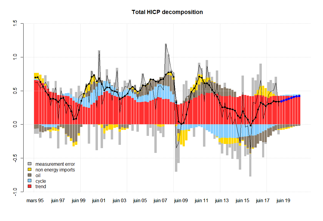
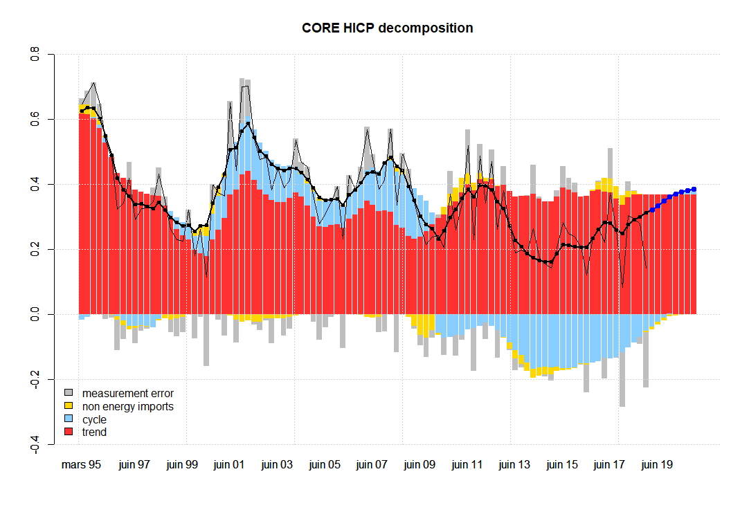
The following graphs represent the two key variables in terms of all the unobserved components specified in the model. The thick black line with dots represents (quarterly) inflation without the measurement error given by the model. Notice that this measurement error in the case of total inflation (first graph), seems to exhibit some level of autocorrelation, while it has been specified as an IID term. In the second graph, corresponding to core inflation, we do not observe autocorrelation in the measurement error at first sight, e.g. see the grey bars, which are the difference between the thick black line with dots and the thin black line.

Structural decomposition and forecasting

These graphs decompose two of the observables (total and core inflation) into the contributions coming from all factors. The blue dots represent out-of-sample forecasts.

Understanding the sources of model misspecification is not an easy task. Some of the possible ways to improve the model without deviating from the rjssf framework are:

• Include some lagged factors in the inflation equation
• Add new variables to better identify the factors (e.g. more indicators related to non-energy related imports, commodities, etc…)
• Add autocorrelation in the measurement errors (e.g. if you want to take seriously the notion that the inflation series is a bad measurement of the underlying inflation)
• Adding more indicators related to inflation expectations

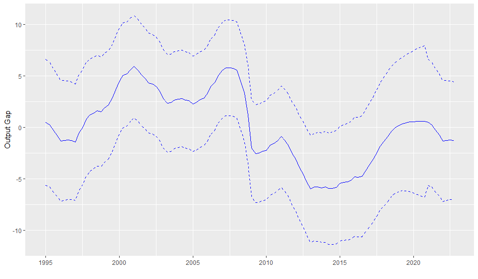
Ploting the unobserved components

One can also look at the unobserved components themselves. The picture below represents the smoothed value of \(\textcolor{blue}{\delta_{t}}\) conditional con the estimated parameters, and a 95$\%$ confidence interval given by the smoothed variance.

[insert code]