Regression-based temporal disaggregation
Introduction
The regression-based temporal disaggregation is defined by the following model:
\[y_t = X_t \beta + \mu_t\]under the constraint that $\mathbf {y_T}=\sum_{t \in T} y_t$. The residuals may be modelled as
| Model | Residuals |
|---|---|
| Chow-lin | $\mu_t = \rho \mu_{t-1}+\epsilon_t$ |
| Fernandez | $\mu_t = \mu_{t-1}+\epsilon_t$ |
| Litterman | $\left(\mu_t-\mu_{t-1}\right) = \rho \left(\mu_{t-1}-\mu_{t-2}\right)+\epsilon_t$ |
The models can be initialized in different ways:
- Chow-lin:
- 0-initialization: $\mu_0=0$
- Unconditional: $\mu_0 \sim N\left(0, \sigma^2/\left( 1-\rho^2\right)\right)$
- Fernandez:
- 0-initialization: $\mu_0=0$
- Diffuse: $\mu_0 \sim N\left(0, k\sigma^2 \right), k\rightarrow \infty$
- Fixed unknown: $\mu_0=\tilde \gamma$
- Litterman:
- 0-initialization: $\mu_0=\mu_{-1}=0$
- Diffuse: $\mu_{-1} \sim N\left(0, k\sigma^2 \right), k\rightarrow \infty \quad \left(\mu_0 - \mu_{-1}\right) \sim N\left(0, \sigma^2/\left( 1-\rho^2\right)\right)$
- Fixed unknown: $\mu_0=\tilde \gamma \quad \mu_{-1}=\tilde \gamma_{-1}$
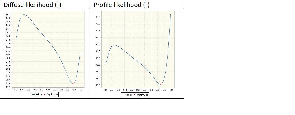
Different choices concerning the initial conditions will lead to different covariance structures for the disaggregated series and usually to different likelihood functions and to different MMSE estimates. However, it should be noted that the Fernandez method with diffuse initialization and the Fernandez method with 0-initialization and mean correction are strictly equivalent. As for the initial residuals, the regression coefficients can be treated in two ways. They can be considered as fixed unknown or they can have an initial diffuse distribution. The likelihood functions based on those hypotheses will differ and lead to different ML estimates of the parameter of the model ($ρ$). It should be noted that the hypothesis on the coefficients of the regression has no direct impact on the MMSE estimates of the disaggregated series.
Details on the likelihood function following the different hypotheses can be found in DK (2001) or in Franke (2010). An example of the impact of that hypothesis on the likelihood function is presented below.
State space forms
Though direct matrix computation could be used, JD+ uses state space forms for estimating the usual temporal disaggregation models. They are described below (see also the generic state space form for temporal disaggregation and benchmarking).
Chow-Lin
State vector
\[\alpha_t=\begin{pmatrix}\mu_t^{\underline C} \\ \mu_t \end{pmatrix}\]Initialization
\[a_{-1} = \begin{pmatrix} 0 & 0\end{pmatrix}\] \[B = \begin{pmatrix} 0 \\ 0 \end{pmatrix}\] \[P_*= \begin{pmatrix} 0 & 0 \\ 0 & 1/\left( 1-\rho^2\right)\end{pmatrix}\]Dynamics
\[T_t =\begin{cases} \begin{pmatrix} 0 & 0 \\ 0 &\rho \end{pmatrix} \text{ if } {t+1}\text{ mod } c = 0 \\ \begin{pmatrix} 0 & 1 \\ 0 & \rho\end{pmatrix} \text{ if } t\text{ mod } c = 0 \\\begin{pmatrix} 1 & 1 \\ 0 & \rho \end{pmatrix} \text{ otherwise} \end{cases}\] \[V_t= \begin{pmatrix} 0 & 0 \\ 0 & 1\end{pmatrix}\] \[S_t = \begin{pmatrix} 0 \\ 1 \end{pmatrix}\]Measurement
\[Z_t = \begin{cases} \begin{pmatrix} 0 & 1 \end{pmatrix} \text{ if } {t}\text{ mod } c = 0 \\ \begin{pmatrix} 1 & 1 \end{pmatrix} \text{ if } {t}\text{ mod } c \neq 0\end{cases}\]Fernandez
Fernandez is identical to Chow-Lin, provided that $\rho$ is replaced by $1$ and that the initial conditions are defined by:
\[a_{-1} = \begin{pmatrix} 0 & 0\end{pmatrix}\] \[B = \begin{pmatrix} 0 \\ 1 \end{pmatrix}\] \[P_*= \begin{pmatrix} 0 & 0 \\ 0 & 0 \end{pmatrix}\]